
Inside XLF: The Complete Financial Investment Framework

This essay tries to answer three questions: How does the financial sector actually make money? How should each sub-sector be valued? And what does this peculiar 2026 window mean? Read sequentially or jump to whatever interests you.
Table of Contents
I. The U.S. Financial System and the Composition of XLF
II. Rate Transmission and Money Market Mechanics
III. From Macro to P&L: How Profit Flows Through Each Sub-Sector
IV. Valuation Frameworks: Nine Different Yardsticks
V. Deep Dives on Core Holdings (Based on Q1 2026 Earnings)
VI. The Trump Administration’s Regulatory Paradigm Shift
VII. Trade Timing: Macro Signals and Tactical Framework
VIII. Scenario Analysis and Allocation Strategy
I. The U.S. Financial System and the Composition of XLF
1. What is XLF
The Financial Select Sector SPDR Fund (XLF) holds every financial sector constituent of the S&P 500, roughly 76-80 securities. As of April 9, 2026, the industry weights are: banks ~28.68%, financial services (including payments) ~27.99%, capital markets ~25.51%, insurance ~13.48%, consumer finance ~4.34%.
The structural character of XLF can be summarized in three points. First, large banks plus payment networks form the foundation: banks contribute spread income and credit elasticity, while card networks and payment infrastructure provide stable fee-based cash flows that are insensitive to rates but sensitive to consumption and cross-border flows. Second, the sector is highly sensitive to the macro environment: historical research shows financials underperform during recessions and outperform during recoveries. Third, regulation and capital constraints act as hidden leverage. Marginal changes in stress tests, capital buffers, and capital rule proposals get amplified through dividend and buyback capacity, asset expansion ability, and risk appetite.
2. The Nine Sub-Sectors
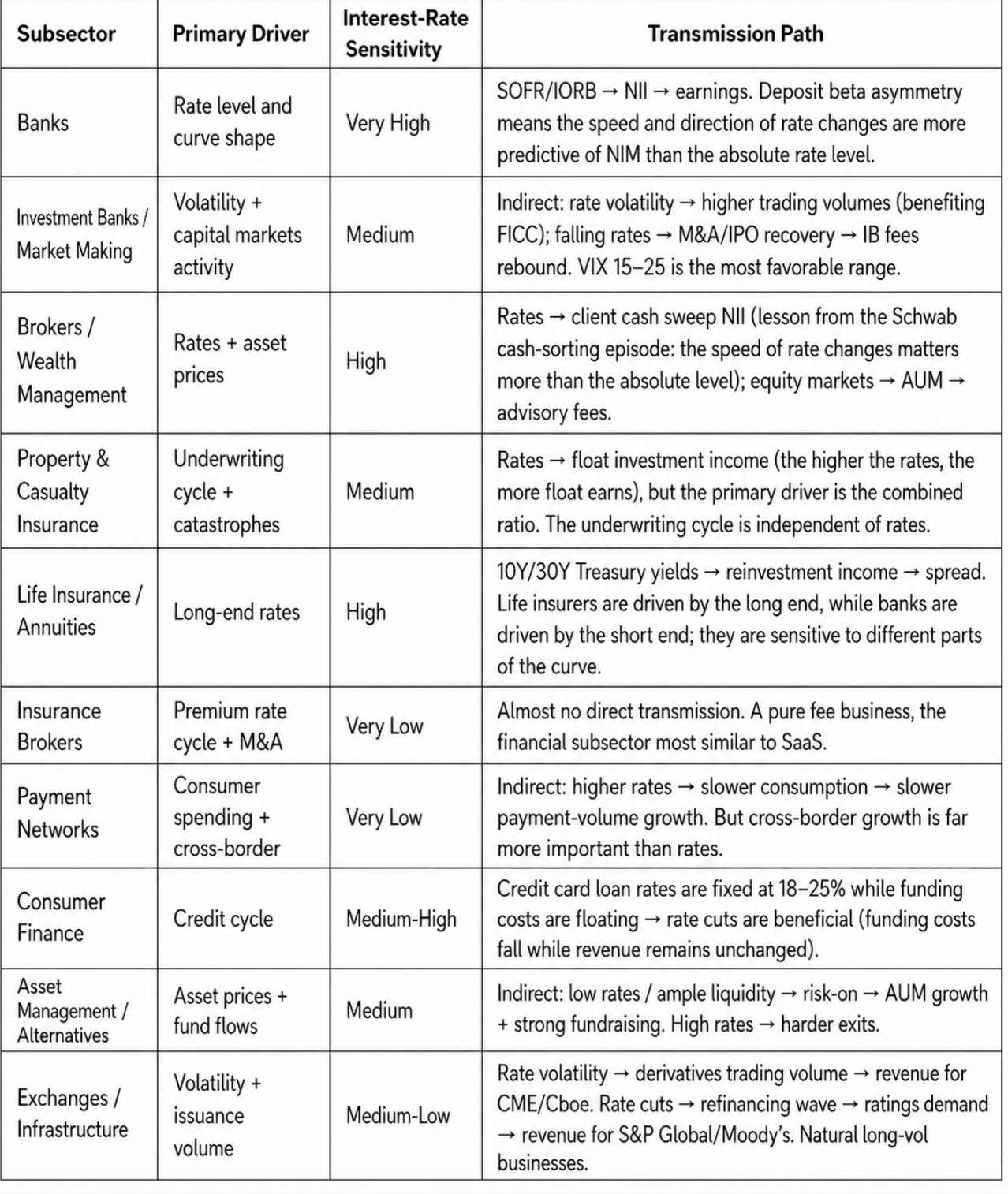
XLF spans at least nine sub-sectors with fundamentally different business models. Profit drivers, rate sensitivity, and cyclical patterns each differ in nature. Understanding this segmentation is critical—going long XLF and going long banks are two completely different bets.
1. Diversified Money Center Banks — JPM, BAC, C, WFC. Run commercial banking (deposit/loan NII), investment banking (advisory + underwriting), trading (FICC + Equities), and wealth management simultaneously. Broadest revenue base, exposed to both rate cycles and capital market activity.
2. Investment Banks and Capital Markets — GS, MS. Revenue centered on trading and IB, with 60-70% from non-NII businesses. Limited rate sensitivity but extreme exposure to M&A cycles and IPO pipelines.
3. Regional and Consumer Banks — USB, PNC, Truist, M&T Bank, etc. Mostly traditional spread businesses, with minimal IB or trading. Purer exposure to NII and local credit quality. CRE concentration (Commercial Real Estate Concentration) runs much higher than at money center banks—it measures bank exposure to commercial real estate (offices, malls, multifamily, etc.) and was the core issue behind the 2023 regional bank crisis.
4. Consumer Finance / Credit Cards — AXP, COF, SYF. Extremely high credit spreads (loan APRs of 18-25% minus funding costs of 4-5%) but also high credit losses (charge-off rates of 3-8%), making them highly cyclical to consumer credit. AXP is the exception due to its affluent customer base.
5. Payment Networks — Visa (V), Mastercard (MA). Combined weight ~13.5%. Zero credit risk, zero rate sensitivity, 50-65% net margins. Essentially a toll road on consumer spending. Cross-border volume growth (+14-20%) is the core engine.
6. Asset Management — BlackRock (BLK), Blackstone (BX), KKR, Apollo (APO), ARES. Revenue formula: AUM × fee rate. Drivers are market beta and net inflows. The industry is caught between fee compression and alternative-asset expansion. The “management fee (durable) + carry (cyclical)” framework maps onto macro regimes: low rates and easy liquidity favor fundraising and valuations; high rates and tight credit pressure exits and marks first.
7. Brokers / Wealth Management Platforms — Schwab (SCHW), Robinhood (HOOD), Ameriprise (AMP). Three legs: client cash NII spread, advisory fees, and transaction-related revenue. Rate sensitivity sits between banks and asset managers.
8. Insurance — Three sub-categories:
P&C (PGR, CB, TRV, ALL, ACGL): Earn underwriting profit + float investment income. Drivers are combined ratio and rates (which affect float yield). Underwriting cycle is independent of the banking cycle.
Life / Annuity (MET, PRU, AFL): Earn premium spread and investment returns. Highly sensitive to long-end rates—higher rates make new annuity guarantees easier to cover.
Insurance Brokers (AON, AJG, WTW): Pure fee businesses—help corporates buy insurance, earn commissions/fees, with zero underwriting risk. Driven by organic growth + M&A. High margins, strong cash flow, low cyclicality, and accordingly much richer valuations (25-30x P/E vs 10-13x for banks).
9. Exchanges and Financial Infrastructure — CME, ICE, CBOE, Nasdaq, S&P Global (SPGI), MSCI, Moody’s (MCO). Revenue from transaction fees, data subscriptions, index licensing, and ratings. Toll-booth-style fee models with strong network effects and high pricing power, with margins of 50%+.
3. Scale and Infrastructure of the U.S. Financial System
The U.S. financial system is a composite of: the banking system (deposits, loans, payment accounts) + the capital markets (direct financing and risk pricing) + financial infrastructure (payment clearing and securities settlement) + a multi-headed regulatory framework (functional regulation + institutional regulation + consumer protection + systemic risk coordination).
On scale: U.S. commercial bank total assets are $25.26 trillion across 4,336 commercial banks and savings institutions. JPMorgan alone holds 17.4% of industry assets ($4.4 trillion). Industry NIM hit 3.39% in Q4 2025 (highest since 2019); community bank NIM 3.77%. Unrealized securities losses dropped sharply from $481 billion in Q4 2024 to $306 billion in Q4 2025 (lowest since Q1 2022), mainly because 30-year mortgage rates fell during the quarter, lifting MBS values. North American asset managers control $88.2 trillion of AUM—63% of the global top-500 total of $139.9 trillion. Daily U.S. equity volume averages 12.2 billion shares. Annual credit card spending: $5.5 trillion. U.S. insurance net premiums: ~$1.7 trillion.
Financial infrastructure determines how financial activity actually settles. Large-value transfers run on Fedwire (final settlement using Fed accounts) and the privately-operated CHIPS (netting with liquidity savings). Bulk retail payments go through ACH networks (rules set by Nacha). Post-trade central depository and settlement is handled by DTCC and its subsidiaries: DTC as the central securities depository, NSCC as the equity clearing and netting hub, settling on T+1.
For investors this means: the U.S. financial sector isn’t a single industry but a multi-layered profit system built on deposit, securities, payment, clearing, ratings, and data networks. The same macro variable typically only matters to a subset of these sub-sectors.
4. Six Major Regulators
Federal Reserve: Central bank, monetary policy maker, primary regulator of bank holding companies; runs the annual stress tests and Basel capital framework. OCC: Charters and supervises national banks and federal savings institutions. FDIC: Deposit insurance ($250K per depositor cap). SEC: Investor protection, fair and efficient markets, capital formation. CFPB: Consumer Financial Protection Bureau (created by Dodd-Frank, drastically weakened under Trump). CFTC: Derivatives markets. Plus FINRA (broker-dealer SRO) and FSOC (systemic risk coordination council).
This is why valuing financial stocks isn’t just about the rate cycle—you also need to track the regulatory perimeter, because capital requirements, consumer protection, M&A approval standards, and market rules each affect different business models in different ways.
II. Rate Transmission and Money Market Mechanics
To understand financial stocks—especially banks—you have to understand how the Fed converts a single rate number in a press release into the actual price of every transaction in the market. That mechanism is called the Interest Rate Corridor, and it’s the pricing infrastructure for the entire financial system.
1. Why a Corridor? The Shift from Quantity Control to Price Control
Before the 2008 crisis the Fed used a completely different system. Reserves earned no interest (IORB was zero), and there was no ON RRP. The Fed controlled rates by precisely managing the quantity of reserves through open market operations. Too many reserves and banks weren’t short of cash, so the interbank rate fell. Too few reserves and banks were short, so it rose. The New York Fed’s trading desk had to forecast each morning’s reserve demand and use Treasury purchases or sales to fine-tune the quantity, steering Fed Funds toward target. The precision required was enormous—a few billion too many or too few in reserves and the rate could miss target.
After QE, reserves swelled from hundreds of billions to trillions, and this “quantity control” model became unworkable. The Fed couldn’t move rates by tweaking a few billion in a system already drowning in liquidity. So it invented the corridor: regardless of total reserves, as long as you set the floor and ceiling, market rates stay framed inside. Reserves can be $3 trillion or $4 trillion—as long as they don’t fall below “ample,” the corridor functions.
The same backdrop explains why required reserve ratios have been completely abandoned in the U.S. The Fed cut required reserves to zero in March 2020 and never restored them. This wasn’t a temporary pandemic measure—it was an acknowledgment of reality: in an ample-reserves framework, reserve requirements no longer function as a binding tool. Bank lending isn’t “find reserves first, then lend”—it’s “lend first, create deposits, then find reserves to satisfy requirements.” And Basel III’s LCR (Liquidity Coverage Ratio) and NSFR (Net Stable Funding Ratio) functionally replaced the prudential role of reserve ratios with something more comprehensive than a simple “keep X% of deposits as reserves.” Note: the PBOC still uses RRR cuts as a regular policy tool (currently around 7%), because China’s financial system relies heavily on bank deposit funding and has relatively underdeveloped capital markets, making the RRR a still-effective “big-pipe” quantitative tool.
2. The Four-Layer Corridor
The current Fed Funds target range is 3.50%-3.75%. The Fed uses four tools to box market rates inside this range:
Layer 1: ON RRP (3.40%) — The Absolute Floor of the Money Market
ON RRP (Overnight Reverse Repurchase Agreement) is a deposit facility the Fed offers to non-bank financial institutions like money market funds (MMFs).
Example: you run a $50 billion MMF. A securities dealer asks to borrow overnight at 3.35% via repo. Do you lend? No—you can park the same money in ON RRP at 3.40% with the Fed as counterparty and zero credit risk. So you either decline or demand more than 3.40%. That sets the absolute floor for short-term funding rates.
Why a dedicated facility for MMFs? Because money funds aren’t banks, don’t have Fed accounts, and can’t earn IORB. Before ON RRP existed, MMFs could only buy T-Bills, lend in repo to dealers, or buy commercial paper. ON RRP gave them a direct channel to transact with the Fed: hand cash to the Fed, receive a Treasury as overnight collateral, get cash plus interest back the next day. The ON RRP rate is typically set 10bps below the lower bound of the target range.
ON RRP balance changes are an important liquidity signal. ON RRP peaked at $2.5 trillion in 2023 and has now drawn down to near zero as the Fed shrank its balance sheet and Treasury issued more T-Bills. The exhaustion of ON RRP means the easiest liquidity buffer in the financial system has been depleted. When Treasury used to issue heavily, MMFs could pull cash out of ON RRP to fund the buying without affecting reserves; now that ON RRP is nearly empty, MMFs buying new T-Bills have to source cash from elsewhere, which eventually pulls from reserves.
Layer 2: IORB (3.65%) — The Bank’s Opportunity-Cost Anchor
IORB (Interest on Reserve Balances) is what the Fed pays commercial banks on reserves held at the Fed.
Example: you’re Bank A, and Bank B asks to borrow overnight at 3.60%. Do you lend? No—you can leave that money at the Fed and earn 3.65% risk-free. So you either decline or demand more than 3.65%.
But Bank B isn’t dumb either—it also has a Fed account. If market rates exceed 3.65%, Bank B is better off using its existing reserves than borrowing expensive cash in the market. So in equilibrium, interbank lending rates don’t drift far from IORB.
From an individual bank’s perspective, IORB is its reservation rate—the bank won’t lend below it, so it looks like a floor. But in actual markets, EFFR typically prints a few basis points below IORB (currently ~3.58% vs IORB 3.65%). Why?
Because of access restrictions. Not every financial institution can earn IORB—only depository institutions with Fed reserve accounts (commercial banks, thrifts, credit unions, U.S. branches of foreign banks). Crucially, the following are excluded:
Government-Sponsored Enterprises (GSEs): Fannie Mae, Freddie Mac, and the Federal Home Loan Banks (FHLBs). FHLBs sit on tens of billions of cash that earns zero at the Fed.
Money Market Funds (MMFs): hold trillions but aren’t banks and have no reserve account.
Non-bank entities of primary dealers: the non-bank legal entities of Goldman, JPMorgan IB arms don’t earn IORB.
These access restrictions create an arbitrage opportunity:
If FHLBs have $20 billion of idle cash earning zero at the Fed, and a bank offers to borrow it at 3.60%, FHLBs will of course lend—earning something beats earning nothing. The commercial bank borrows at 3.60% and immediately deposits it at the Fed to earn IORB 3.65%—a risk-free 5bps. This arbitrage drags EFFR down to roughly 3.58-3.60%, below IORB but above ON RRP.
So IORB’s accurate description is “the anchor for EFFR”—neither a hard ceiling nor a hard floor, but a magnetic level that pulls market rates toward it. EFFR sits a few bps below IORB because of the GSE arbitrage. If everyone could earn IORB, IORB would be the only floor needed. Precisely because some can’t, the Fed had to build a multi-layer corridor.
Layer 3: Discount Window / SRF (3.75%) — The Ceiling
The Discount Window is the Fed’s oldest tool (dating back to 1913). Any depository institution with a Fed account can use it: pledge eligible collateral (Treasuries, MBS, loan portfolios) to its regional Federal Reserve Bank and borrow at the discount rate. The current discount rate is 3.75%, exactly the upper bound of the Fed Funds target range.
But the Discount Window’s biggest problem is stigma. Historically, once the market learns a bank used the Discount Window, it gets read as “this bank can’t borrow in the market and is going to the central bank for emergency liquidity”—which can trigger confidence collapse or even a run. So in normal times, banks would rather pay slightly higher rates in the market than touch the Discount Window.
The SRF (Standing Repo Facility), established in 2021, is the lower-stigma alternative. The SRF lets primary dealers and designated banks pledge Treasuries to the Fed for overnight cash at the upper bound of the Fed Funds target range (3.75%). The core problem the SRF solves isn’t bank cash shortage—it’s dealer cash shortage. When dealers hold Treasuries but can’t convert them to cash, the entire repo market seizes up.
Example: the September 2019 repo crisis. Corporate tax payments and a heavy Treasury settlement window simultaneously drained liquidity, and overnight repo rates spiked from ~2% to 10% in a few hours. Had the SRF existed, cash-short dealers could have gone directly to the SRF for funding at the upper-bound rate, and rates wouldn’t have run away. The SRF’s existence is itself a form of insurance—if traders know there’s a backstop near 3.75%, they don’t panic-bid rates higher. The tool’s existence matters more than its actual use (announcement effect).
Key differences between SRF and Discount Window: target audience (Discount Window → banks; SRF → primary dealers); stigma level (SRF designed as a routine tool); collateral scope (Discount Window accepts a very broad set including loan portfolios; SRF accepts only Treasuries and agency MBS).
If the Fed wants to hike 25bps, it just shifts all administered rates in lockstep: ON RRP from 3.40% → 3.65%, IORB from 3.65% → 3.90%, Discount/SRF from 3.75% → 4.00%. The whole corridor translates upward, and EFFR and SOFR follow automatically. Setting the level of short-term rates no longer requires daily fine-tuning of reserve quantity through open market operations, the way it did before 2008.
3. SOFR: The Real Pricing Yardstick
SOFR (Secured Overnight Financing Rate) is the ballast of today’s global financial markets. EFFR is more of a small-circle interbank print, while SOFR is the actual funding price underpinning the entire financial system.
What SOFR is: not a Fed-administered rate, but the volume-weighted median of actual overnight repo transactions collateralized by U.S. Treasuries. The New York Fed publishes the prior day’s SOFR each business morning at 8 a.m. The data come from three categories of overnight repo:
Tri-party Repo: the largest sub-market. BNY Mellon serves as agent; MMFs and GSEs are the largest cash providers, sitting on trillions of idle cash whose only outlet besides ON RRP is the repo market.
GCF Repo (General Collateral Finance): dealer-to-dealer trades cleared through DTCC’s FICC, used to balance positions or fund Treasury inventory.
Bilateral Repo (DVP Repo): trades between hedge funds and primary dealers. Hedge funds pledge Treasuries to borrow cash for leveraged longs (or pledge cash to borrow specific Treasuries for shorts). This piece is the most volatile and is what occasionally pushes SOFR up.
Scale comparison: SOFR daily volume is $1.8-2.1 trillion, nearly 20x EFFR (~$100bn/day). Why such a gap? Because in the modern financial system, no one likes unsecured credit lending (EFFR); secured lending against Treasuries (SOFR) is the dominant form.
Why SOFR replaced LIBOR: LIBOR was based on bank submissions (manipulable—the 2012 scandal saw multiple major banks fined billions), while SOFR is based on actual transactions and Treasury-collateralized (essentially zero credit risk). By mid-2023, SOFR fully replaced LIBOR as the core benchmark in the U.S. financial system. Now nearly every floating-rate financial contract is anchored to SOFR: corporate floating-rate loans (SOFR + credit spread), hundreds of trillions of dollars of global interest rate swaps, adjustable-rate mortgages (ARMs), some student loans, and floating-rate credit cards.
SOFR’s place in the corridor: SOFR is indirectly bracketed by ON RRP and SRF. If repo rates fall below ON RRP (3.40%), MMFs park cash at ON RRP rather than in repo, preventing SOFR from falling further. If repo rates surge near SRF (3.75%), dealers go to the SRF for cash, capping SOFR. In normal conditions, SOFR runs slightly above ON RRP and near IORB—currently around 3.55-3.60%.
Why is SOFR below IORB but banks still participate in the repo market? On the surface this seems contradictory: a bank can earn 3.65% (IORB) at the Fed, so why lend at 3.58% (SOFR) in repo? Three reasons:
First, banks are often borrowers in the repo market, not lenders. Large banks borrow cash from repo (SOFR ~3.58%) and immediately deposit it at the Fed to earn IORB 3.65%—a risk-free 5-7bps. SOFR being below IORB is good news for banks: they can absorb cheap funding from MMFs and pocket the Fed spread.
Second, sometimes a bank lends cash at a low rate to obtain scarce Treasury collateral. When a specific Treasury is in tight supply (e.g., the most recently issued 10-year is heavily shorted), a bank might lend cash below IORB to acquire that hot Treasury and re-lend it elsewhere at a higher rate. This is “specials repo,” where rates can drop to near zero or even negative because the collateral itself is more valuable than the interest.
Third, regulatory capital efficiency (netting). Banks frequently run two-sided books in repo—e.g., lend $5bn to a hedge fund (receive Treasuries) while simultaneously borrowing $5bn from an MMF (post Treasuries). If both trades clear through FICC’s central counterparty, they can be netted on the balance sheet under accounting rules: $5bn assets and $5bn liabilities offset to near-zero net, and the SLR denominator barely budges. By contrast, simply parking $5bn at the Fed adds $5bn to balance sheet assets, increases the SLR denominator by $5bn, with nothing to net against. The SLR denominator is total assets, not risk-weighted—reserves and Treasuries may be zero-risk, but each dollar still consumes leverage capital just like junk loans. So banks would rather give up a few bps of spread (running below IORB in repo) in exchange for a leaner balance sheet, more SLR headroom, and freed-up capital for higher-yielding businesses (lending, market-making, etc.).
SOFR’s signal value: in normal conditions, SOFR moves only 1-2bps day-to-day. If SOFR suddenly spikes 10-20bps (occasionally happens at quarter-end or year-end as banks shrink balance sheets), it means repo market liquidity is tightening and reserves may be approaching the “no longer ample” threshold. A narrowing IORB-SOFR spread (SOFR rising toward IORB) signals tight funding; a widening spread (SOFR pressed lower, away from IORB) signals abundant cash. SOFR breaking above IORB is an unambiguous liquidity-shortage alarm.
4. Reserves, Quantitative Tightening, and the Leverage Chain
What reserves are
Reserves are funds that banks hold in their Fed accounts. After the required reserve ratio was cut to zero in March 2020, banks hold reserves entirely voluntarily—because IORB pays interest (currently 3.65%), reserves are zero credit risk, zero duration risk, 100% liquid assets that simultaneously satisfy LCR and other regulatory requirements.
As of April 2026, total banking system reserves are about $3.3 trillion, and the Fed’s balance sheet is about $6.7 trillion. SOMA holds about $6.4 trillion in securities ($4.2 trillion Treasuries + $2.2 trillion MBS).
How QT and TGA affect reserves
When Treasuries on the Fed’s balance sheet mature, they’re not fully rolled (the monthly cap was cut from $25bn to $5bn starting April 2025, sharply slowing QT, and QT is now paused). Maturing principal pulls cash out of the banking system.
Key mechanism: when ON RRP balances were still high (e.g., $2 trillion+ in 2023), QT primarily drained ON RRP rather than reserves—MMFs pulled cash out of ON RRP to buy newly issued T-Bills, and reserves were unaffected. But ON RRP is now near zero, so QT now drains reserves one-for-one. That’s why the Fed sharply slowed QT in April 2025—to avoid pushing reserves to the “no longer ample” threshold and breaking the corridor.
TGA (Treasury General Account), the Treasury’s account at the Fed, is another disturbance variable. When Treasury issues heavily or it’s tax season, large flows move from banks into TGA, and reserves temporarily fall. When Treasury spends, the cash flows back to banks and reserves rise. TGA fluctuates between $325bn and $950bn, and a hundreds-of-billions move can create violent short-term reserve swings. In 2025, the debt ceiling pushed TGA down to about $325bn at one point; once the ceiling was raised, it refilled rapidly. That’s why every Treasury auction and every tax window can trigger money market volatility.
The leverage chain: from reserves to retail
To understand why reserves matter, you have to understand the entire leverage chain of the financial system. The Fed is the ultimate liquidity source, and leverage propagates down the funding chain layer by layer:
Fed (ultimate source) → Large banks (obtain reserves from the Fed and fund in wholesale markets) → Hedge funds (obtain leverage through prime brokerage and repo) → Brokers (obtain funding from banks and provide margin loans to retail) → Clearinghouses (backed by bank credit lines, provide leverage to futures and options traders) → PE funds (obtain leverage through syndicated loans and disperse it through CLOs to insurers and pension funds).
When reserves shrink → bank funding costs rise → banks raise repo and prime brokerage rates to hedge funds → hedge fund funding costs rise → low-yielding leverage strategies (like Treasury basis trades, where 50x leverage earns just a few bps) become uneconomic first → funds are forced to cut positions → asset selling pressure rises → volatility spikes → margin calls cascade → not just hedge funds, but retail margin accounts also get topped up or force-liquidated. That’s the deleveraging spiral.
5. Banks’ Balance Sheets and Treasuries: A Deeper Relationship
Banks don’t buy Treasuries as a simple “investment”—it’s the core of asset-liability management. Securities portfolios typically make up 20-25% of total bank assets, split into three accounting buckets:
Trading Book: held by IB and market-making desks, marked-to-market daily into the income statement. Smaller in size, but volatility hits current earnings directly.
Available-for-Sale (AFS): securities the bank may sell before maturity. Marked-to-market, with unrealized gains/losses flowing through AOCI directly into shareholders’ equity. The 2022 rate hikes drove unrealized AFS losses above $200bn industrywide. For the 9 Advanced Approaches banks (JPM, BAC, C, GS, MS, etc.), AFS unrealized losses must flow through CET1 regulatory capital—rising rates not only eat book equity but also drag down regulatory capital ratios. In 2015, other banks were given a one-time choice to remove AOCI from regulatory capital (the “opt-out”), and most took it.
Held-to-Maturity (HTM): carried at amortized cost, immune to mark-to-market swings. But if a bank is forced to sell HTM early, it must reclassify the entire HTM portfolio as AFS and recognize all unrealized losses in one shot. Both SVB in 2023 and Republic First Bank in 2024 died from this mechanism: $15bn of hidden losses sat off the balance sheet, deposit runs forced sales, and the banks failed within 48 hours.
As of Q4 2025, industry unrealized securities losses had fallen to $306bn (down sharply from $481bn in Q4 2024, the lowest since Q1 2022)—mostly because 30-year mortgage rates fell during the quarter, lifting MBS values.
Banks play three roles in the Treasury market: primary dealer (24 Primary Dealers required to participate in every Treasury auction), Treasury secondary market maker (~$700-800bn daily volume), and one of the largest Treasury buyers (banks hold ~$4.5-5 trillion of Treasuries and agencies for ALM and HQLA requirements).
The significance of eSLR reform: SLR requires banks to hold capital against total assets (not risk-weighted assets). Treasuries carry zero risk weight in the risk-weighted framework, but under SLR they consume leverage capital just like any other asset. Each dollar of Treasuries a bank buys adds zero credit risk but increases the SLR denominator. The November 2025 final eSLR rule replaced the fixed 2% buffer with “half of GSIB Method 1 surcharge,” releasing approximately $384bn of excess Tier 1 capital. If Treasuries are eventually fully exempted from the SLR denominator, it would substantially expand banks’ capacity to hold and make markets in Treasuries—critical given the explosion in Treasury issuance ($36 trillion outstanding, $8-10 trillion annual issuance).
6. Macro Drivers Across Sub-Sectors
The rate machinery above (IORB, SOFR, ON RRP, the yield curve) hits banks most directly because banks’ core profit model is the spread itself—rate changes immediately move both sides of the NII equation. But the other XLF sub-sectors have different first-order drivers, which we’ll unpack in detail in the next section
.
III. From Macro to P&L: How Profit Flows Through Each Sub-Sector
We’ve established how the rate corridor works and mapped the macro sensitivities of each sub-sector. But how does a macro event like “rates down 50bps” actually travel, step by step, into the billions of extra NII on JPMorgan’s income statement? When Visa’s cross-border volume grows 14%, how does the money move from a cardholder’s pocket to Visa’s P&L?
1. Banks
Banks’ NII = earning-asset yield × earning-asset volume − interest-bearing liability cost × interest-bearing liability volume. Simple on the surface, but the transmission mechanism has two critical nonlinear features.
Deposit Beta Asymmetry
Deposit beta measures how sensitive deposit rates are to changes in the benchmark rate. If the Fed cuts 100bps, how much do bank deposit rates fall?
The key fact: deposit beta is asymmetric across hiking and cutting cycles. In a hiking cycle, deposit rates are sticky upward but flexible downward—banks are reluctant to raise deposit rates, and they delay as long as possible. During the 2022-2023 hiking cycle, large bank deposit betas were roughly 40-50% (the Fed hiked 525bps, but deposit rates only rose about 200-250bps). In a cutting cycle, however, banks can slash deposit rates very quickly.
Walk through what a 100bps Fed cut actually does:
Asset side (reprices relatively quickly): floating-rate loans (roughly 40% of the loan book, priced at SOFR + spread) drop almost immediately by 100bps. Fixed-rate loans (roughly 60%) are completely unaffected until they mature and reprice. Weighted average asset yield falls about 40-50bps.
Liability side (reprices even faster): demand deposits (checking accounts, 30-40% of deposits) are already near zero and can’t be cut further. But CDs get rolled at lower rates when they mature; money market deposit accounts (MMDAs) can be repriced quickly. Weighted average funding cost falls about 50-60bps.
NIM change: liabilities reprice down 10-20bps more than assets, so NIM actually expands.
This is precisely why, after the Fed cut 175bps in 2024-2025, industry NIM rose from 3.22% to 3.39% (highest since 2019). The FDIC explicitly attributed it to “funding costs falling faster than earning-asset yields.”
The flip side: NIM initially gets compressed in a fast-hiking cycle. When the Fed started hiking in March 2022, floating-rate loan yields jumped immediately, but deposit rates lagged—NIM should have expanded. The problem was that once rates rose high enough, depositors started moving cash out of low-rate accounts and into money market funds (because MMF rates track Fed Funds closely while sweep rates don’t). Banks were forced to reprice deposits higher or borrow expensive replacement funding from the FHLBs and wholesale markets. That’s Schwab’s cash sorting crisis—we’ll cover it in detail in the broker section.
Takeaway for bank stock positioning: don’t simply assume “rate cuts hurt banks, rate hikes help banks.” What actually matters is the speed-and-direction combination. Slow rate cuts are best for banks (funding costs fall quickly while assets reprice slowly). Fast hikes help initially but carry late-cycle deposit outflow risk. Fast cuts can compress NIM short-term (assets reprice first) but improve it medium-term.
The Fixed-Rate Asset Repricing Snowball
This is the strongest structural tailwind for bank NII growth right now.
In the ultra-low-rate environment of 2020-2021, banks originated massive volumes of fixed-rate mortgages, MBS, and long-term bonds yielding only 2-3%. These assets have stated maturities of 15-30 years, but effective duration (accounting for prepayments) of roughly 5-7 years. That means about 15-20% of the low-rate fixed-rate book matures or prepays each year, and banks can reinvest the proceeds at today’s much higher rates.
Example: BAC holds about $900bn in fixed-rate assets. Assume $150bn (roughly 17%) matures in 2026, originally yielding 2.5%, reinvested at the current 4.5%. That single repricing produces $150bn × (4.5% − 2.5%) = $3bn of additional annualized NII. That’s exactly what BAC management means when they say “fixed-rate asset repricing” is the primary NII growth driver, and it’s the foundation for BAC’s guidance of NII growing another 5-7% in 2026.
This effect runs for years because the 2020-2021 low-rate stock is enormous—each year a fresh batch matures and generates another tranche of incremental NII. As long as the Fed doesn’t cut rates back to zero, the snowball keeps rolling.
2. Investment Banks
IB revenue engines work nothing like banks—not spreads, but activity, volatility, and volume.
Market-Making Bid-Ask Spreads and VIX
Market makers earn the bid-ask spread. What happens when VIX rises from 12 to 25?
Spreads widen: uncertainty increases, market makers carry more inventory risk and demand wider spreads as compensation. A large-cap stock’s bid-ask might go from one cent to three to five cents.
Volume explodes: volatility forces investors to reposition—hedge funds hedge, pensions rebalance, retail stops out or buys dips. Average daily volume might double.
Double leverage: spreads 2-3x wider × volume 2x = trading revenue can spike 4-6x. That’s why GS Q1 2025 Equities hit a record $4.19bn—tariff panic spiked volatility and simultaneously widened spreads and lifted volume.
But VIX above 35-40 turns negative: market liquidity dries up, market makers can get caught holding inventory on the wrong side in a sharp one-way move, and trading losses offset spread income.
For most full-service investment banks, moderate-to-elevated but not out-of-control volatility is the ideal environment—wide enough spreads, high enough client activity. But if volatility surges further into a liquidity crunch, inventory risk and risk-limit constraints bite back against trading revenues.
Prime Brokerage Financing Spreads and SOFR
Large banks finance hedge funds through prime brokerage at SOFR + a credit spread, with the spread depending on fund size, strategy risk, and negotiating leverage. A large multi-strategy fund might pay SOFR + 40-80bps; a small single-strategy fund might pay SOFR + 150-250bps.
This is the fastest-growing and most stable part of Equities. Of MS’s $15.6bn in Equity revenues for 2025, financing and prime brokerage contributed about 40-45% ($6-7bn)—bigger and more durable than market-making.
Key transmission: when SOFR rises, if a bank’s funding cost (SOFR) and client lending rate (SOFR + spread) rise in lockstep, the spread is unchanged and NII is unaffected. But if competition compresses the spread, NII falls. Conversely, when market volatility rises, hedge fund demand for leverage increases, prime balances grow, and even with unchanged spreads, the larger book drives revenue. Citi’s prime balances grew over 50% in 2025 from exactly this dynamic.
IB Advisory Pipeline and CEO Confidence
M&A advisory fees are the highest-margin IB business (near-zero marginal cost) but also the most cyclical. M&A activity depends on:
CEO confidence: corporate leaders only pursue large acquisitions when they’re optimistic about the economic outlook and comfortable with valuations. The relationship with rates is indirect—rates affect discount rates and financing costs, which in turn affect deal economics and feasibility.
Credit conditions: leveraged buyouts require banks to provide bridge loans and leveraged loans. When credit markets are loose (HY OAS low) and banks are willing to lend, LBO activity picks up.
Announced-but-not-closed pipeline: M&A typically takes 6-12 months from announcement to close. So current advisory fee revenue reflects deals announced 6-12 months ago. This means IB fees are a lagging indicator—you see the M&A pipeline revive and then wait another half year before it shows up in reported earnings.
Global M&A was up 36% year-over-year in 2025, and GS booked $9.34bn in full-year IB fees. If 2026 brings further deregulation + rate cuts + CEO confidence recovery, M&A could accelerate further.
The Cross-Sell Multiplier
A single M&A mandate at a full-service investment bank simultaneously triggers 5-6 revenue streams:
Financing: bridge loan → leveraged loan → DCM underwriting
Hedging: interest rate and FX exposure on the deal → FICC derivatives
Market-making uplift: target company stock volume explodes after announcement → Equities market-making revenue
Wealth management: founder/executive personal wealth management → WM advisory fees
Follow-on: post-merger capital structure optimization, secondary offerings, buybacks
A boutique advisory firm (Evercore, Lazard) earns only the advisory fee itself. A full-service platform like JPM or GS generates 3-5x the total revenue per transaction. That’s the structural advantage of the universal bank model.
3. Brokers
Schwab’s 2022-2024 cash sorting crisis is the best textbook for understanding the broker business.
The Mechanism
A broker’s NII comes from the spread on client idle cash. When a client holds $50,000 of idle cash in their Schwab account, Schwab sweeps that cash to its own bank subsidiary or a partner bank, which deploys it into Treasuries or loans and earns the market rate (say, 4.5%), but only pays the client a very low sweep rate (say, 0.45%). The 4.05% spread is Schwab’s NII.
This model works perfectly when rates are low. Clients don’t care whether their idle cash earns 0% or 0.1%, since money market funds are also paying 0.1%. But when the Fed hiked from 0% to 5.25% in just 16 months starting March 2022, the model blew up.
The Crisis
March 2022: the Fed begins hiking. MMF rates quickly follow Fed Funds to 4-5%, but Schwab’s sweep rate remains 0.45%.
Late 2022 through 2023: clients begin moving sweep cash en masse into money market funds. Schwab’s bank deposits fell from a Q1 2022 peak of $466bn to a Q2 2023 trough of $304bn—over $162bn drained. During the fastest drawdown period from August 2022 to April 2023, outflows ran about $5.6bn per month.
Supplemental funding: Schwab was forced to borrow heavily from FHLBs and the short-term CD market at 4.5-5% to replace the lost low-cost deposits. Bank Supplemental Funding peaked above $80bn.
NIM collapse: the original model—borrow at 0.45%, earn 4.5% on Treasuries (NIM ~4%)—was replaced by borrow at 4.5%, still earn 4.5% on Treasuries (NIM near zero). NIM bottomed at 2.07%.
Stock collapse: SCHW fell from ~$90 early 2022 to ~$45 at the 2023 low—cut in half.
The Recovery
By end of 2025: with 175bps of Fed cuts, money market fund yields fell and some cash flowed back into sweep accounts. Supplemental funding fell from $80bn+ to $5.1bn. NIM recovered to 2.90%. Revenue hit a record $23.9bn.
Schwab and similar platform brokers earn a core profit from converting client idle cash into low-cost liabilities and capturing the spread. The model is extremely robust in low-rate environments, but in a fast-hiking cycle, clients become much more sensitive to the gap between sweep rates and money market yields, triggering cash migration and a spike in replacement funding costs. If next-generation AI financial tools further reduce client tolerance for rate differentials, this pressure may no longer be purely cyclical—it could become partly structural.
4. Insurance
The P&C Profit Formula
P&C insurer profit = underwriting profit + float investment income.
Underwriting profit = net premiums × (1 − combined ratio). Combined ratio = loss ratio + expense ratio. Below 100% means underwriting profit.
Example: Berkshire’s GEICO posted a combined ratio of 81.5% in 2024. Assuming net premiums of $45bn, underwriting profit = $45bn × (100% − 81.5%) = $8.3bn. That means for every dollar of premium collected, only $0.815 was spent on claims and operations.
Float investment income: insurers collect premiums before paying claims (often months to years later), and in the interim the float compounds. Berkshire’s float stands at $171bn. At current short-term Treasury yields of roughly 3.5-4%, that $171bn of float generates about $6-7bn in annualized investment income—and the float costs zero or even negative (if underwriting is profitable, the implied cost of the float is actually negative).
The Dual-Boost Effect of Higher Rates on P&C
When rates rise:
Float investment income increases: $171bn × each 100bps in rates = an additional $1.7bn in annualized income.
Underwriting discipline is typically unaffected: premium pricing is based on actuarial models (expected claims + expenses + profit margin), not rates.
So a high-rate environment is doubly good for P&C: underwriting profit and investment income improve simultaneously. That’s why 2023-2025 (high rates + hard market underwriting cycle) was the golden era for P&C insurers. Travelers’ underwriting profit went from $2.1bn in 2022 → $3.2bn in 2023 → $4.5bn in 2024 → $5.5bn in 2025—2.5x in four years.
The Underwriting Cycle: Independent of the Economic Cycle
Insurance has its own underwriting cycle:
Soft market (competition phase): capital floods into insurance → premiums fall → combined ratios rise → some players exit at a loss → supply shrinks → transition to hard market. Typically lasts 3-5 years.
Hard market (discipline phase): after a major loss event, insurers exit markets and survivors reprice → premiums grow strongly → combined ratios fall → profits surge → new capital enters → competition intensifies → transition back to soft market. Typically lasts 2-4 years.
2023-2025 was the mid-to-late stage of a hard market, with strong premium growth partially offset by rising catastrophe frequency (climate change).
Life/Annuity vs. P&C: Different Rate Drivers
Life insurance watches the long end (10Y/30Y Treasury yields); P&C watches the short end (T-Bills/SOFR).
Why: life insurers have extremely long-duration liabilities (policy claims may come 30-50 years later), requiring long-duration fixed income assets to match. When the 30-year yield moves from 2% to 4.5%, the reinvestment yield on new investments nearly doubles—a structural, multi-year profit improvement for life insurers, analogous to the fixed-rate asset repricing effect at banks.
P&C has short-dated claims (auto insurance claims typically settle within 6-12 months), so float is invested in short-term Treasuries and commercial paper, making P&C more sensitive to short-end rates.
